Quickstart: command-line interface with YAML
This tutorial will show you how to use immuneML for a simple machine learning analysis on an adaptive immune receptor repertoire (AIRR) dataset. This example dataset consists of 100 synthetic immune repertoires (amino acid sequences generated by OLGA), each containing 1000 CDR3 sequences. In half the repertoires, the subsequence ‘VLEQ’ has been implanted in 5% of the CDR3 sequences to simulate a disease signal. Using immuneML, we will encode the data as 3-mer frequencies and train a logistic regression model to predict the disease status of each repertoire (i.e., whether the repertoire contains the disease signal ‘VLEQ’), which is a binary classification problem.
Getting started using the command-line interface
This tutorial assumes that immuneML is already installed locally (see Installing immuneML). We recommend installing immuneML using a package manager.
Step 0: test run immuneML
This is an optional step. To quickly test out whether immuneML is able to run, try running the quickstart command:
immune-ml-quickstart ./quickstart_results/
This will generate a synthetic dataset and run a simple machine machine learning analysis on the generated data.
The results folder will contain two sub-folders: one for the generated dataset (synthetic_dataset) and one for the results of the machine
learning analysis (machine_learning_analysis). The files named specs.yaml are the input files for immuneML that describe how to generate the dataset
and how to do the machine learning analysis. The index.html files can be used to navigate through all the results that were produced.
Step 1: downloading the dataset
An archive containing the dataset used in this tutorial can be downloaded here: quickstart_data.zip.
It contains the following files:
The 100 repertoire_<somenumber>.tsv, which are immune repertoire files in AIRR format. For details about the AIRR format, see the AIRR documentation and this example file).
A metadata.csv file. The metadata file describes which of the 100 repertoires are diseased and healthy, under the column named ‘signal_disease’ which contains the values True and False. For details about the metadata file, see What should the metadata file look like? and this example file
Step 2: writing the YAML specification
Any immuneML analysis is described by a YAML specification file.
This file contains nested key-value pairs. Mandatory keywords with a specific meaning are styled like this
in the text. Note that correct whitespace (not tab) indentation of the YAML file is important.
In this tutorial, we will only cover the essential elements of the YAML specification. For a more complete introduction, see How to specify an analysis with YAML.
The YAML specification consists of:
definitionsdescribing the analysis components.datasets: our data is in AIRR format, we need to provide the location of the repertoires and the metadata file.encodings: the data will be represented through a k-mer frequency encoding. This means each repertoire is represented based on the frequency of subsequences of length k. For example, the sequence CSVQYF contains the 3-mers CSV, SVQ, VQY and QYF.ml_methods: we will use logistic regression to classify the encoded immune repertoires.Optionally,
reports: we will plot the coefficients of the trained logistic regression model, to get more insight into what the model has learned.
instructionsdescribing the type of analysis.The TrainMLModel instruction is used to train one or more ‘ML settings’ (combinations of encodings and ML methods), and optimize the hyperparameters using nested cross-validation. We can set the parameters for the outer ‘assessment’ and inner ‘selection’ cross-validation loops.
The complete YAML specification for this analysis is shown below and can be downloaded here: quickstart.yaml.
Make sure to change path/to/repertoires/ and path/to/metadata.csv to the actual paths to the data on your local machine.
definitions:
  datasets:
    my_dataset: # user-defined dataset name
      format: AIRR
      params:
        is_repertoire: true # we are importing a repertoire dataset
        path: path/to/repertoires/          # path to the folder containing the repertoire .tsv files
        metadata_file: path/to/metadata.csv

  encodings:
    my_kmer_frequency: # user-defined encoding name
      KmerFrequency:   # encoding type
        k: 3           # encoding parameters

  ml_methods:
    my_logistic_regression: LogisticRegression # user-defined ML model name: ML model type (no user-specified parameters)

  reports:
    my_coefficients: Coefficients # user-defined report name: report type (no user-specified parameters)

instructions:
  my_training_instruction: # user-defined instruction name
    type: TrainMLModel

    dataset: my_dataset # use the same dataset name as in definitions
    labels:
    - signal_disease    # use a label available in the metadata.csv file

    settings: # which combinations of ML settings to run
    - encoding: my_kmer_frequency
      ml_method: my_logistic_regression

    assessment: # parameters in the assessment (outer) cross-validation loop
      reports:  # plot the coefficients for the trained model
        models:
        - my_coefficients
      split_strategy: random   # how to split the data - here: split randomly
      split_count: 1           # how many times (here once - just to train and test)
      training_percentage: 0.7 # use 70% of the data for training

    selection: # parameters in the selection (inner) cross-validation loop
      split_strategy: random
      split_count: 1
      training_percentage: 1 # use all data for training

    optimization_metric: balanced_accuracy # the metric to optimize during nested cross-validation when comparing multiple models
    metrics: # other metrics to compute for reference
    - auc
    - precision
    - recall

    number_of_processes: 4 # processes for parallelization
Step 3: running the analysis
Once the YAML specification has been saved to a file (for example: quickstart.yaml), the analysis can be run using the following steps:
Activate the virtual environment where immuneML is available.
Navigate to the directory where
quickstart_specs.yamlwas saved.Run the following command:
immune-ml quickstart_specs.yaml ./quickstart_results/
Step 4: understanding the results
The results folder contains a multitude of files and folders, which can most easily be navigated by opening ./quickstart_results/index.html in a browser.
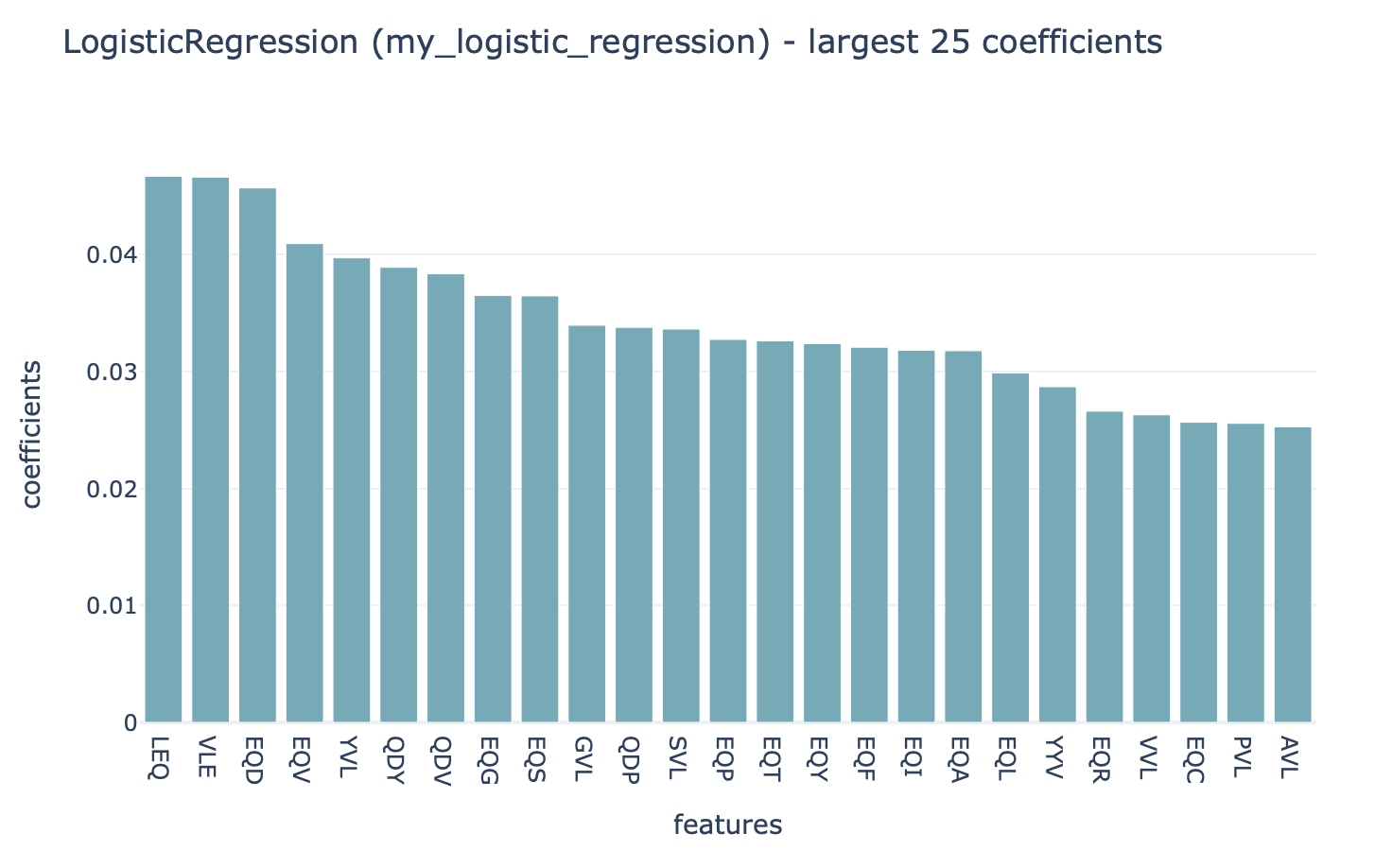
This HTML page displays a summary of the analysis, the performance of the optimized ML model (click ‘see details’ to navigate further), and the report that plots the 25 top coefficients of
the trained logistic regression model. Notice how the coefficients with the highest values are associated with the k-mers ‘VLE’ and ‘LEQ’, which overlap with the implanted disease signal ‘VLEQ’, meaning the ML model learned the correct signal.
In the folder ./quickstart_results/exported_models/ a .zip file can be found containing the configuration of the optimal ML settings, including settings for the encoding
and machine learning method. Using immuneML, these optimal ML settings can subsequently be applied to a new repertoire dataset with unknown disease labels.
The folder ./quickstart_results/my_training_instruction/ contains all raw exported results of the TrainMLModel instruction including all ML model predictions and raw report results.
Finally, ./quickstart_results/ contains the complete YAML specification file for the analysis and a log file.
What’s next?
If you haven’t done it already, it is recommended to follow the tutorial How to specify an analysis with YAML. If you want to try running immuneML on your own dataset, be sure to check out How to import data into immuneML. Other tutorials for how to use each of the immuneML Galaxy tools can be found under Tutorials. You may also be interested in checking our Use case examples to see what else immuneML can be used for.